AP Microeconomics Factor Markets (Unit 5): Why MRP and Derived Demand Trip Up Students Who Aced Units 1-4


Serious About Your AP Scores? Let’s Get You There
From understanding concepts to scoring 4s and 5s, EduShaale’s AP coaching is built for results — with personalised learning, small batches, and exam-focused strategy.
10-13% Unit 5's share of the 60-question MCQ section -- the lowest of any tested unit | ~6-8 Class periods College Board suggests for the whole unit -- also the least of any unit | 19% Of AP Microeconomics test-takers scored a 5 in 2026 (College Board) | 4 Required topics: factor markets intro, demand/supply shifts, competitive hiring, monopsony |
MP x MR The single formula every hiring decision in this unit comes back to | 30-50% Of AP Micro free-response points require drawing or reading a graph | 1 Guaranteed short free-response question on Unit 5 in the Personal Progress Check | 127K Students sat the AP Microeconomics exam in 2026 (College Board) |

Table of Contents
Introduction: The Unit That Breaks a Four-Unit Winning Streak
What Unit 5 Actually Is -- Understanding AP Microeconomics Factor Markets
How Much Unit 5 Is Actually Worth on the AP Microeconomics Exam
Derived Demand: The Idea Every Other Concept in This Unit Depends On
Marginal Revenue Product (MRP): Definition, Formula, and Worked Calculations
Graphing Factor Markets: The Diagrams That Actually Show Up on the FRQ
Seven Mistakes That Cost Students Points on Factor Market Questions
Worked Practice Problems: Six Factor Market Calculations, Solved
Introduction: The Unit That Breaks a Four-Unit Winning Streak
By the time students reach Unit 5, most have built real momentum. Units 1 through 4 reward the same recurring habits -- read a graph, compare a marginal figure to a price, find where two curves cross -- and students who have drilled those habits are, by this point in the course, often scoring well on unit tests. Then factor markets arrive, and the pattern breaks. College Board's own course framework is unusually direct about this: it describes factor markets as "one of the biggest challenge areas for students on the AP Exam," and identifies the exact reason why -- the unit sits near the end of the course, carries the joint-lowest exam weighting of any unit, and consequently gets rushed by students and teachers who treat a small percentage as a small workload.
That trade-off is not a safe one to make. AP Microeconomics Factor Markets is not a harder version of the supply-and-demand graph from Unit 2 -- it is a role reversal. In every product-market unit so far, the firm has been the seller. In Unit 5, the firm becomes the buyer: it buys labour, capital, and land from households, and the households become the sellers. Every graph, every axis label, and every optimisation rule a student has memorised for product markets has to be rebuilt for this new direction, and the AP Exam is written on the assumption that most students will not do that rebuilding carefully.
The result shows up in a specific, predictable way: strong students correctly calculate marginal product, correctly identify a profit-maximising rule, and then apply the wrong version of it -- confusing marginal revenue product with marginal product, assuming a firm's position in its output market determines its position in the labour market, or reading a monopsony wage off the wrong curve. None of these are conceptual gaps in the traditional sense. They are transfer errors, made by students who understood marginal analysis perfectly well four units ago.
This guide works through Unit 5 the way it actually needs to be learned: what factor markets are and why the buyer/seller roles flip, the derived-demand logic that drives every subsequent formula, the exact mechanics of marginal revenue product (MRP) and marginal resource cost (MRC), the profit-maximising hiring rule, and the perfectly competitive-versus-monopsony comparison that anchors most Unit 5 free-response questions. It includes three fully labelled graphs, six worked numerical problems, a seven-item myth list built directly from where students actually lose points, a complete formula sheet, and a short study plan scaled to the single week most courses actually spend on this unit.
1. What Unit 5 Actually Is -- Understanding AP Microeconomics Factor Markets
Every unit before this one studied a product market: a market where firms sell output -- goods and services -- and households buy it. Unit 5 studies the mirror image, a factor market (also called a resource market or input market), where the roles reverse. Firms become the buyers. Households become the sellers. What gets bought and sold is not a finished good but a factor of production -- something firms need in order to produce that finished good.
College Board's course framework defines three factors of production for this unit, each paid through a specific factor price:
Factor of Production | Who Supplies It | Payment It Earns |
Labour | Households (workers) | Wages |
Capital | Households (savers/investors) | Interest |
Land | Households (landowners) | Rent |
The core flip: In a product market, the firm sets a price and decides how much to sell. In a factor market, the firm is the one paying a price -- the wage, the interest rate, or the rent -- and deciding how much to buy. Every graph in this unit has to be built from the firm's perspective as a buyer, not a seller. |
The clearest way to see why this trips up strong students is to look at what stays the same and what changes. The underlying logic of the unit is identical to every profit-maximising rule taught since Unit 1: compare a marginal benefit to a marginal cost, and keep going until they are equal. What changes is the direction. A firm hiring labour asks, "does one more worker add more revenue than they cost?" -- the same marginal-benefit-versus-marginal-cost comparison as Unit 3's output decision, run in reverse, against a different pair of curves, on a graph with different axes.
College Board is explicit that this combination -- familiar logic applied in an unfamiliar direction, tested near the end of the course when review time is shortest -- is exactly why factor markets underperforms relative to how well most students actually understand marginal analysis. Its own guidance to teachers warns that the unit's light weighting invites exactly this kind of rushing, and recommends treating factor markets explicitly as an application of ideas already learned -- supply and demand, and marginal analysis -- rather than as a new topic to be crammed in at the end.
2. How Much Unit 5 Is Actually Worth on the AP Microeconomics Exam
Factor markets carries the joint-lowest weighting of any unit on the multiple-choice section -- but "low weighting" does not mean "safe to skip," and the free-response section treats it very differently from the multiple-choice section. Here is how all six units compare, straight from the current AP Microeconomics Course and Exam Description:
Unit | Name | Exam Weighting | Suggested Class Periods |
1 | Basic Economic Concepts | 12-15% | 9-11 |
2 | Supply and Demand | 20-25% | 13-15 |
3 | Production, Cost, and the Perfect Competition Model | 22-25% | 11-13 |
4 | Imperfect Competition | 15-22% | 8-10 |
5 | Factor Markets | 10-13% | 6-8 |
6 | Market Failure and the Role of Government | 8-13% | 9-11 |
Two things stand out. First, Unit 5 gets the least classroom time of any unit in the course -- six to eight 45-minute periods, against nine to fifteen for every other unit. Second, despite that light footprint, Unit 5 is not optional on the exam: the Personal Progress Check for this unit is built from roughly 10 multiple-choice questions and one free-response question, and factor-market reasoning regularly gets folded into the larger, multi-part free-response questions that anchor Section II.
That free-response section is where the unit's real weight shows up. Across the whole AP Microeconomics exam, drawing or reading an accurately labelled graph accounts for 30 to 50% of all free-response points -- the single largest task category on the exam -- and factor-market graphs are among the most distinctive on the entire syllabus, because they are the one place students must plot wage against quantity of labour instead of price against quantity of output. A student who has the concepts right but reaches for the wrong axis labels under exam pressure can lose graphing points on a question they otherwise understood completely.
Exam Component | Timing | Points / Weighting | Where Unit 5 Shows Up |
Section I -- Multiple Choice | 70 minutes, 60 questions | 66.65% of score | ~6-8 questions drawn directly from Unit 5 content |
Section II, Q1 -- Long FRQ | Part of 60 min (+10 min reading) | 10 points | Often combines a product-market graph with a factor-market graph in one question |
Section II, Q2/Q3 -- Short FRQ | Part of 60 min (+10 min reading) | 5 points each | Frequently the dedicated factor-market question in a given year |
The practical takeaway: treat the 10-13% multiple-choice figure as a scheduling fact, not a signal about depth. A unit that guarantees a Personal Progress Check free-response question and regularly reappears inside a 10-point long FRQ is worth the same rigorous treatment as any other unit -- it simply needs less calendar time to get there.
3. Derived Demand: The Idea Every Other Concept in This Unit Depends On
Every demand curve studied before this unit came from consumer preferences -- households wanted a good for its own sake, and demand followed directly from that want. Labour demand does not work this way. A firm does not hire a data analyst because it enjoys employing data analysts; it hires one because analysts help produce something the firm can sell. This is derived demand: the demand for a factor of production is derived from -- comes second-hand from -- the demand for the output that factor helps produce.
Derived demand has exactly two moving parts, and every factor-demand question on the exam traces back to one or both of them:
The resource's productivity -- how much extra output one more unit of the factor produces (its marginal product). A more productive worker or a more efficient machine is worth more to hire, holding everything else constant.
The value of the output -- what that extra output actually sells for. A worker producing the same physical quantity of goods is worth hiring at a higher wage when the output price rises, because each unit of what they produce is now worth more.
Put those two together and you get the exact logic behind the unit's core formula, covered in the next section: the demand for labour is driven by how much labour produces and by what that production is worth in the output market -- nothing else. A rise in consumer demand for coffee does not directly increase the demand for baristas; it raises the price of coffee, and that price increase is what raises the value of hiring another barista. The consumer's preference matters only insofar as it moves the output price.
Why this matters for the whole unit: Every subsequent topic -- MRP, the hiring rule, monopsony -- assumes derived demand as the starting point. If a factor-demand question ever seems to depend on "consumers wanting more of it" as a standalone cause, trace it back to one of the two derived-demand drivers above before answering. Consumer taste for the final good is not, by itself, a valid reason for a factor demand curve to shift. |
4. Marginal Revenue Product (MRP): Definition, Formula, and Worked Calculations
Marginal revenue product (MRP) turns derived demand into a number. It is the additional revenue a firm earns from employing one more unit of a resource -- the dollar-value answer to "what is hiring one more worker actually worth to this firm?"
MRP Formula MRP = MP x MR MP = marginal product (the extra output from one more unit of the input, in physical units). MR = marginal revenue (the extra revenue from selling one more unit of output). MRP is always measured in currency, never in physical units. |
This single formula splits into two cases, and the exam expects students to know which one applies before calculating anything:
When the output market is perfectly competitive
Marginal revenue equals price (MR = P), because a perfectly competitive firm can sell any quantity at the going market price. Substituting into the formula gives a special case with its own name -- the value of the marginal product (VMP):
VMP -- the perfectly-competitive special case VMP = MP x P (equal to MRP only when MR = P) This is the version most introductory examples use, and the one that is easiest to over-apply. |
When the output market is imperfectly competitive
Marginal revenue is below price and falling as output rises -- the same MR-below-demand relationship from the Unit 4 monopoly graph. Because MRP uses MR, not P, MRP falls faster than it would under perfect competition -- diminishing marginal product pulls it down, and declining marginal revenue pulls it down again on top of that. Using price instead of marginal revenue here overstates what an extra worker is actually worth to the firm, which is precisely the error the worked example below is built to catch.
Worked example: MRP under perfect competition
A firm sells its output at a constant price of $20 per unit (a perfectly competitive product market). Its short-run production data:
Workers | Total Product | Marginal Product (MP) | MRP = MP x $20 |
1 | 10 | 10 | $200 |
2 | 19 | 9 | $180 |
3 | 27 | 8 | $160 |
4 | 34 | 7 | $140 |
5 | 40 | 6 | $120 |
6 | 45 | 5 | $100 |
Because price is constant, MRP falls here for one reason only: diminishing marginal product. This is also the firm's labour demand curve -- read straight off the MRP column, it already shows how many workers the firm would hire at any given wage.
Worked example: MRP under imperfect competition (the VMP trap)
Now suppose the same firm instead faces a downward-sloping demand curve for its own output:
Output (Q) | Price (P) | Total Revenue (TR) | Marginal Revenue (MR) |
4 | $30 | $120 | -- |
5 | $28 | $140 | $20 |
6 | $26 | $156 | $16 |
If hiring a sixth worker raises output from 5 to 6 units (MP = 1 unit), the correct MRP calculation uses marginal revenue, not price:
Correct: MRP = MP x MR = 1 x $16 = $16. This is the true value of hiring the sixth worker. |
Common error (produces VMP, not MRP): MP x P = 1 x $26 = $26. This overstates the worker's value by $10, because it ignores that selling one more unit also pushed the price down on every unit already being sold. VMP only equals MRP when the output market is perfectly competitive. |
The single most important fact in this section: The MRP curve is the firm's demand curve for that input. It slopes downward for the same reason a product-market demand curve for a normal good behaves the way it does -- but the mechanism is diminishing marginal product (and, under imperfect competition, falling marginal revenue on top of it), not diminishing marginal utility. |
Need a structured plan instead of going it alone? EduShaale's 1-on-1 AP Microeconomics coaching walks through MRP, MRC, and monopsony graphing exactly in the sequence used in this guide, built around your existing course calendar. Book a free 60-minute strategy session -> |
5. The Profit-Maximising Hiring Rule: MRP = MRC
Hiring one more unit of a resource makes sense as long as it earns more than it costs. That comparison has a name on each side: the benefit side is MRP, covered above; the cost side is marginal resource cost (MRC) -- sometimes called marginal factor cost (MFC) -- the extra cost of employing one more unit of the resource.
The Profit-Maximising Hiring Rule Hire additional units of a resource as long as MRP > MRC. Stop hiring at the point where MRP = MRC. This is the exact same logic as the Unit 3 output rule (produce while MR > MC, stop where MR = MC) -- run against a different pair of curves, in the opposite market direction. |
What MRC actually equals depends entirely on the structure of the factor market -- and this is where the unit's single most consequential distinction sits.
In a perfectly competitive factor market
Many firms compete to hire the same type of labour, no single firm is large enough to influence the wage, and the firm is a wage taker: it can hire as many or as few workers as it wants at the going market wage, so MRC = wage, and MRC is constant (a horizontal line) for that individual firm -- even though the market labour supply curve is upward-sloping.
Two separate classifications, not one: A firm's position in its output market and its position in its factor market are independent facts about that firm. College Board's course framework makes this point directly: a firm can be a perfect competitor in the labour market while simultaneously being an imperfect competitor in its own output market. A monopolist selling its output can still be a wage taker when it hires workers, and a firm competing intensely on price can still be the dominant employer in a small town. Always answer two separate questions -- "who sets the output price here?" and "who sets the wage here?" -- before assuming one from the other. |
Because MRP = wage at the hiring point, the rule collapses to a simpler, exam-favourite version in this specific case: hire until MRP = wage. A firm keeps hiring as long as the next worker's MRP exceeds the market wage, and stops the moment MRP falls to the wage rate.
The least-cost input rule
Firms typically hire more than one type of input at once -- labour and capital, for instance -- and the same marginal logic extends to choosing the right combination of both. A firm minimises cost (or, equivalently, gets the most output for its spending) when the last dollar spent on every input buys the same additional output:
Least-Cost Input Combination Rule MP(labour) / Price(labour) = MP(capital) / Price(capital) If one ratio is higher than the other, the firm gets more output per dollar from that input -- it should shift spending toward it until the two ratios are equal. |
| |
| This is not a new idea -- it is Unit 1's utility-maximising rule, relabelled: Consumers maximise utility by equalising marginal utility per dollar across the goods they buy (MUx/Px = MUy/Py). Firms minimise cost by equalising marginal product per dollar across the inputs they buy. Same structure, same reasoning, different subject. | |
6. Perfectly Competitive Factor Markets vs Monopsony
A monopsony is a factor market with a single buyer of the resource -- the labour-market mirror of a monopoly. The word is unfamiliar to most students the first time they meet it, but the underlying idea is not: a single large employer in a small town, a hospital system that is the only significant employer of nurses in a region, or a single processor buying an entire area's raw milk are all classic monopsony examples.
Feature | Perfectly Competitive Factor Market | Monopsony |
Number of buyers | Many -- no single firm affects the wage | One -- the firm is the entire demand side |
Firm's labour supply curve | Horizontal (flat) at the market wage | Upward-sloping -- the same curve as the market |
MRC vs wage | MRC = wage (constant) | MRC > wage, and rises faster than supply |
Why MRC behaves that way | Hiring one more worker does not change the wage | Hiring one more worker raises the wage paid to every existing worker, not just the new hire |
Hiring rule | Hire where MRP = wage | Hire where MRP = MRC (a smaller quantity than competitive) |
Wage actually paid | Read directly from the wage line | Read off the supply curve at the profit-maximising quantity -- below MRP and below the competitive wage |
The reason MRC outruns the wage under monopsony is entirely mechanical, and a small numeric version makes it concrete before the full worked problem in Section 10:
Why MRC > wage under monopsony: Suppose 5 workers are willing to work for $10/hour, and attracting a 6th requires raising the wage to $11/hour -- but a single employer cannot pay the 6th worker $11 while paying the other five $10; the wage is the same for everyone. Raising pay to $11 for all six workers costs an extra $1 x 6 = $6, not $1. The 6th worker's true marginal resource cost is $6, even though the wage only rose by $1. |
Applying MRP = MRC under monopsony therefore produces a hiring quantity below what a competitive labour market would generate, and -- because the wage is read off the supply curve at that lower quantity, not off MRC -- a wage below what those same workers would earn in a competitive market. This is the standard monopsony result: fewer workers hired, at a lower wage, than the competitive benchmark, even though each of those workers is still generating more marginal revenue than they are paid.
Section 7 graphs this outcome directly, and Section 10 walks the full numerical version.
One further combination is worth knowing because it shows up in released exam questions: a firm's position in the labour market and its position in the output market combine independently, and the combination changes how many workers ultimately get hired. All else equal, the largest quantity of labour is hired when both markets are perfectly competitive -- any monopsony power in the labour market, or any monopoly power in the output market, independently pulls employment below that fully competitive benchmark, because each type of market power restricts a different curve (MRC in one case, MRP in the other) without changing the underlying hiring rule itself.
7. Graphing Factor Markets: The Diagrams That Actually Show Up on the FRQ
Because 30-50% of AP Microeconomics free-response points depend on an accurately labelled graph, and factor-market graphs are the one place the axes genuinely change, this section is worth treating as its own study block rather than skimming as illustration.
Before drawing anything, relabel the axes: Every factor-market graph uses Wage Rate (W) on the vertical axis and Quantity of Labour (L) on the horizontal axis -- never Price and Quantity of Output. Writing these two labels first, before drawing a single curve, prevents the single most common graphing error on this unit: carrying over axis labels from the product-market graph drawn one question earlier. |
Graph 1: A firm hiring in a perfectly competitive labour market

Construction checklist: (1) label the axes Wage Rate and Quantity of Labour; (2) draw the downward-sloping MRP curve -- this is also labelled DL; (3) draw a horizontal line at the market wage, labelled both MRC and SL; (4) mark the intersection as QE; (5) drop a line down to the horizontal axis and across to the vertical axis to label the equilibrium quantity and wage.
Graph 2: Monopsony

Construction checklist: (1) label the axes; (2) draw the upward-sloping market supply curve, labelled SL -- this also serves as the firm's average resource cost curve; (3) draw the MRC curve above and steeper than supply; (4) draw the downward-sloping MRP curve; (5) find QM where MRP crosses MRC; (6) from QM, drop straight down to the supply curve -- not the MRC curve -- to find WM, the wage actually paid.
The single most common monopsony graphing error: Reading the wage off the MRC curve instead of the supply curve at Q. MRP = MRC only determines the quantity of labour hired -- the wage is always a separate, second step, read from the point on the supply curve directly below that quantity. |
Graph 3: Derived demand in action -- a shift in factor demand
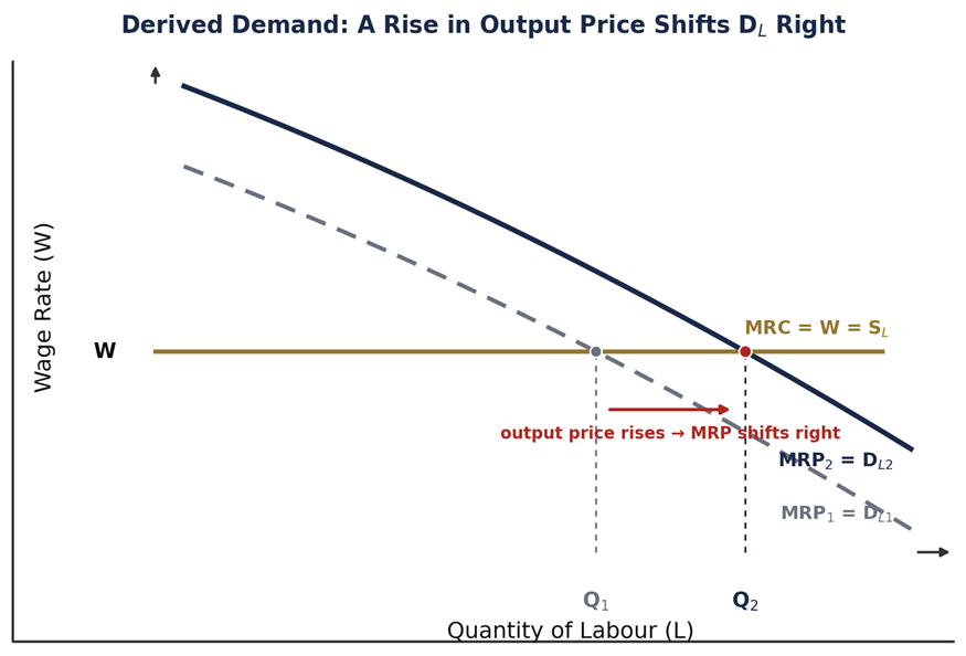
This graph is the visual form of Section 3's derived-demand logic: nothing about worker productivity changed here -- only the value of what workers produce changed, and that alone was enough to shift the whole demand-for-labour curve, raising both the equilibrium wage and quantity hired in a competitive labour market.
8. What Shifts Factor Demand and Factor Supply
Because factor demand is derived demand, its determinants are narrower and different from the determinants of ordinary product demand -- consumer income and tastes do not belong on this list unless they operate through one of the channels below.
Factor Demand Shifter | Direction of Shift | Example |
Output price rises | Demand for the input shifts right | Coffee prices rise -> demand for baristas rises |
Resource productivity (MP) rises | Demand for the input shifts right | Better training raises each worker's output |
Price of a substitute input falls | Demand for this input can shift left | Cheaper machinery reduces demand for the labour it replaces |
Price of a complementary input falls | Demand for this input shifts right | Cheaper software raises demand for the analysts who use it |
Number of firms hiring the input changes | Market demand shifts with the number of buyers | New firms entering an industry raise total labour demand |
Factor Supply Shifter | Direction of Shift | Example |
Immigration / population changes | Labour supply shifts with the size of the workforce | Net inward migration increases local labour supply |
Education and training levels | Supply of qualified workers shifts right as training expands | A new certification programme increases qualified applicants |
Working conditions | Better conditions attract more workers at every wage | Improved safety standards raise supply to that occupation |
Availability of alternative opportunities | More attractive alternatives reduce supply | A booming adjacent industry pulls workers away |
Preferences for leisure vs work | Stronger leisure preference reduces supply at every wage | Shifting cultural attitudes toward work-life balance |
The distinction the exam is actually testing: If a scenario changes what a resource is paid, or how much of it is offered, without going through output price or productivity first, it is a supply-side story, not a demand-side one. Confusing the two is the single fastest way to shift the wrong curve on a factor-market FRQ. |
9. Seven Mistakes That Cost Students Points on Factor Market Questions
None of the errors below come from misunderstanding marginal analysis. Every one of them comes from applying a rule that was correct in an earlier unit to a situation where the direction, the axis, or the underlying assumption has changed.
Myth 1: "Factor markets work just like product markets, only backwards." Truth: The graphs look similar -- an upward-sloping supply curve and a downward-sloping demand curve -- but the axes and the decision rule both change. In a product market, a firm compares price to marginal cost. In a factor market, it compares MRP to MRC, and the firm is the buyer, not the seller. What to do instead: Before drawing any factor-market graph, write "Wage" and "Quantity of Labour" on the axes first, every time. Never carry over Price/Quantity of Output labels from the graph drawn immediately before it. |
Myth 2: "MRP and marginal product (MP) mean the same thing." Truth: MP is measured in physical units of output ("the fourth worker produces seven more units"). MRP is measured in currency (MRP = MP x MR). An MRP answer with no dollar sign is a marginal product answer wearing the wrong label. What to do instead: Label every MRP calculation with a currency symbol. If the final number has no $ in front of it, the calculation stopped one step early. |
Myth 3: "A firm's position in its output market determines its position in its labour market." Truth: These are two separate classifications. College Board states directly that a firm can be a perfect competitor in the labour market while being an imperfect competitor in its output market, or any other combination of the two. What to do instead: Ask two separate questions before graphing anything: "who sets the output price here?" and "who sets the wage here?" Never infer the answer to one from the other. |
Myth 4: "MRC always equals the wage rate." Truth: Only in a perfectly competitive factor market. Under monopsony, MRC is greater than the wage, because hiring one more worker means raising pay for every existing worker at that firm, not only the new hire. What to do instead: Check whether the firm faces a flat (horizontal) labour supply curve or the upward-sloping market supply curve directly. If the firm itself faces the upward-sloping curve, it is a monopsonist, and MRC does not equal the wage. |
Myth 5: "Under monopsony, the wage is wherever MRP equals MRC." Truth: MRP = MRC identifies the profit-maximising quantity of labour only. The wage actually paid is a separate step, read off the labour supply curve at that quantity -- a point below the MRC curve at the same quantity. What to do instead: Use a fixed two-step process every time: (1) find Q where MRP = MRC; (2) drop straight down to the supply curve -- never the MRC curve -- to read the wage actually paid. |
Myth 6: "Factor demand shifts for the same reasons product demand shifts -- income, tastes, prices of related goods." Truth: Factor demand is derived demand. It shifts only when the price of the output changes, the resource's productivity changes, or the price of a related input changes. Consumer taste for the final good matters only to the extent that it moves the output's price. What to do instead: Before shifting a factor demand curve, trace the cause back to one of the derived-demand drivers in Section 3. "Consumers want more of it" is never a complete answer on its own. |
Myth 7: "Since Unit 5 is only 10-13% of the exam, it is safe to skim." Truth: College Board's own course materials warn that this unit gets rushed precisely because of its light weighting and late placement in the course -- and it still guarantees at least one Personal Progress Check free-response question, plus regular appearances inside larger multi-unit free-response questions. What to do instead: Budget at least one full untimed practice session on MRP/MRC calculations, plus one dedicated graphing drill, before moving on. Treat the low multiple-choice weighting as a scheduling fact, not a signal about how much understanding the unit requires. |
10. Worked Practice Problems: Six Factor Market Calculations, Solved
Each problem below mirrors a pattern that shows up repeatedly in released AP Microeconomics free-response questions. Work through the steps before checking the answer.
Problem 1 -- Basic MRP under perfect competition
A firm sells output at a constant $20/unit. A worker's marginal product is 7 units. What is that worker's MRP?
Identify the formula: MRP = MP x MR.
Because the output market is perfectly competitive, MR = P = $20.
MRP = 7 x $20 = $140.
Answer: MRP = $140. |
FRQ-style justification to write: "Since MR equals price in a perfectly competitive output market, MRP equals MP multiplied by price: 7 x $20 = $140."
Problem 2 -- MRP under imperfect competition (avoiding the VMP trap)
A firm faces a downward-sloping demand curve for its output. Increasing output from 5 to 6 units raises total revenue from $140 to $156, while price falls from $28 to $26. What is the MRP of the worker responsible for that sixth unit?
Calculate marginal revenue: MR = change in TR / change in Q = ($156 - $140) / 1 = $16.
The worker's marginal product is 1 unit (output rose by exactly 1 unit).
MRP = MP x MR = 1 x $16 = $16 -- not MP x P (1 x $26 = $26), since MR, not P, applies whenever the output market is imperfectly competitive.
Answer: MRP = $16 (using price instead of marginal revenue would overstate this by $10). |
Problem 3 -- Profit-maximising hiring in a competitive labour market
Using the MRP schedule from Problem 1's firm, and a competitive market wage of $130/hour, how many workers should the firm hire?
Worker | MP | MRP (at P = $20) | Hire? (wage = $130) |
| |
3rd | 8 | $160 | Yes -- MRP > wage |
| |
4th | 7 | $140 | Yes -- MRP > wage |
| |
5th | 6 | $120 | No -- MRP < wage |
| |
| Answer: Hire 4 workers -- the last worker for whom MRP still exceeds the wage. | ||||
Problem 4 -- Monopsony: MRC, hiring quantity, and the wage actually paid
A monopsonist faces this labour supply schedule and this MRP schedule:
Quantity of Labour | Wage (from supply) | Total Labour Cost (Q x Wage) | MRC | MRP |
1 | $10 | $10 | -- | $24 |
2 | $11 | $22 | $12 | $20 |
3 | $12 | $36 | $14 | $17 |
4 | $13 | $52 | $16 | $16 |
5 | $14 | $70 | $18 | $13 |
Find Q where MRP = MRC: at Q = 4, MRP = $16 = MRC = $16. Hire 4 workers.
Find the wage actually paid: read it off the supply column at Q = 4, not the MRC column -- $13/hour, not $16.
Note the gap: the 4th worker generates $16 of MRP but is paid $13. That $3 gap -- captured by the firm rather than paid out -- is the standard monopsony result.
Answer: Hire 4 workers at a wage of $13/hour, even though the 4th worker's MRP is $16. |
Problem 5 -- Least-cost input combination
A firm pays $20/hour for labour (MP = 100 units) and $40/hour to rent capital (MP = 150 units). Is the firm minimising cost? If not, what should it do?
MP(labour) / Price(labour) = 100 / 20 = 5.
MP(capital) / Price(capital) = 150 / 40 = 3.75.
Since 5 > 3.75, the firm earns more output per dollar from labour than from capital -- it is not yet minimising cost.
Answer: Shift spending toward labour and away from capital. Hiring more labour lowers its marginal product (diminishing returns), while using less capital raises its marginal product, until the two ratios are equal. |
Problem 6 -- Derived demand: predicting a shift
The market price of frozen yoghurt rises from $3 to $4 per unit. Worker productivity at frozen-yoghurt shops is unchanged. Predict the effect on the labour market for frozen-yoghurt-shop workers.
Output price is one of the two derived-demand drivers (Section 3); productivity (MP) is unchanged, so the entire effect runs through the output-price channel.
Since MRP = MP x MR, and MR moves with the higher output price in a competitive output market, MRP rises at every quantity of labour.
A rise in MRP at every quantity shifts the entire labour demand curve to the right (see Graph 3, Section 7).
In a competitive labour market, a rightward demand shift with an unchanged supply curve raises both the equilibrium wage and the equilibrium quantity of workers hired.
Answer: Both the equilibrium wage and the quantity of frozen-yoghurt-shop workers hired increase. |
11. The Unit 5 Formula and Quick-Reference Sheet
Term | Formula | What It Means |
Marginal Product (MP) | Change in Total Output / Change in Quantity of Input | Extra output from one more unit of the input |
Marginal Revenue Product (MRP) | MP x MR | Extra revenue from one more unit of the input |
Value of Marginal Product (VMP) | MP x P | MRP specifically when the output market is perfectly competitive (MR = P) |
Marginal Resource Cost (MRC / MFC) | Change in Total Resource Cost / Change in Quantity of Input | Extra cost of hiring one more unit of the input |
Profit-Maximising Hiring Rule | Hire where MRP = MRC | Stop hiring once the next unit costs more than it earns |
Least-Cost Input Rule | MP(L)/P(L) = MP(K)/P(K) | Correct input mix once marginal product per dollar is equal across inputs |
Two labels, one number, only under perfect competition: MRP and VMP are the same number only when the output market is perfectly competitive. Outside a perfectly competitive output market, always use MRP (built from MR); VMP will overstate the true value of the resource. |
12. A Study Plan for the Week You Cover Factor Markets
Most AP Microeconomics courses give this unit six to eight class periods -- roughly a single school week. The plan below is scaled to that window rather than to a multi-week calendar, on the assumption that Units 1-4 are already largely in place.
Day | Focus | Target Before Moving On |
Day 1 | Derived demand, the three factors of production, and the buyer/seller role reversal | Explain in one sentence why factor demand is "derived" rather than direct |
Day 2 | MRP and MP calculations, including the perfect-vs-imperfect-competition MRP/VMP distinction | Complete Problems 1 and 2 from Section 10 without notes |
Day 3 | The profit-maximising hiring rule and the competitive factor-market graph | Draw Graph 1 from memory, correctly labelled, in under 90 seconds |
Day 4 | Monopsony: why MRC exceeds the wage, and the two-step hiring-then-wage process | Complete Problem 4 and draw Graph 2 from memory |
Day 5 | Factor demand and supply shifters, plus the least-cost input rule | Complete Problems 5 and 6 from Section 10 |
Day 6 / Weekend | Full Personal Progress Check 5 (about 10 MCQ and 1 short FRQ) under timed conditions | Self-score the FRQ against the task verbs in Section 7 -- identify, explain, calculate, draw |
If the unit only gets one review session before the exam: Prioritise the monopsony two-step process (Section 6-7) and the MRP-vs-VMP distinction (Section 4) over everything else in this unit. Released free-response questions draw on these two ideas more often than any other Unit 5 content. |
Ready to Start Your AP Journey?
EduShaale’s AP Coaching Program is designed for students aiming for top scores (4s & 5s). With expert faculty, small batch sizes, personalized mentorship, and a curriculum aligned to the latest AP format, we help you build deep conceptual clarity and exam confidence.
Subjects Covered: AP Calculus, AP Physics, AP Chemistry, AP Biology,
AP Economics & more
📞 Book a Free Demo Class: +91 90195 25923
🌐 www.edushaale.com/ap-coaching
Free Diagnostic Test: testprep.edushaale.com
13. Frequently Asked Questions
Q: What is Unit 5 in AP Microeconomics?
Unit 5, Factor Markets, covers how firms buy the resources -- labour, capital, and land -- they need to produce goods and services. It flips the buyer/seller roles from every earlier unit: firms become buyers, and households become sellers of these resources, receiving wages, interest, and rent in return. The unit carries 10-13% of the multiple-choice section and is built around four topics -- introduction to factor markets, changes in factor demand and supply, profit-maximising behaviour in competitive factor markets, and monopsony.
Q: What percentage of the AP Microeconomics exam is factor markets?
Factor markets makes up 10-13% of the 60-question multiple-choice section, tied with Unit 6 for the lowest weighting of any unit. It is not separately broken out as a fixed percentage of the free-response section, but factor-market reasoning appears in the Unit 5 Personal Progress Check (about 10 multiple-choice questions and one short free-response question) and regularly reappears inside larger, multi-unit free-response questions.
Q: What is marginal revenue product (MRP) in simple terms?
MRP is the extra revenue a firm earns by employing one more unit of a resource, such as one more worker. It is calculated as marginal product multiplied by marginal revenue (MRP = MP x MR). Firms use MRP, not marginal product alone, to decide whether hiring one more unit of a resource is actually profitable, because MRP converts physical output into a dollar figure that can be compared directly against the cost of hiring.
Q: What is the difference between MRP and marginal product?
Marginal product (MP) is measured in physical units -- the extra output one more worker produces. MRP is measured in currency -- what that extra output is actually worth in revenue, calculated as MP multiplied by marginal revenue. A common exam error is reporting an MP figure where an MRP figure was asked for, or vice versa; checking whether the answer should carry a currency symbol is a fast way to catch this mistake.
Q: What is derived demand?
Derived demand is the idea that the demand for a resource comes from the demand for whatever that resource is used to produce, rather than from any direct want for the resource itself. A firm's demand for accountants, for instance, depends on the demand for the firm's own product, not on any inherent desire to employ accountants. Derived demand has exactly two drivers: the resource's productivity, and the price of the output it helps produce.
Q: What is the profit-maximising rule for hiring labour?
A firm should hire additional units of a resource as long as the marginal revenue product (MRP) of doing so exceeds the marginal resource cost (MRC), and stop hiring at the point where MRP equals MRC. In a perfectly competitive labour market, MRC simply equals the market wage, so the rule is often stated more simply as "hire until MRP equals the wage."
Q: What is marginal resource cost (MRC), and how is it different from the wage?
Marginal resource cost (MRC), also called marginal factor cost (MFC), is the additional cost of employing one more unit of a resource. In a perfectly competitive labour market, MRC equals the wage rate, because hiring one more worker does not change what the firm pays anyone else. Under monopsony, MRC is greater than the wage, because raising pay to attract one more worker means raising pay for every worker already employed at that wage, not only the new hire.
Q: What is a monopsony, and how is it different from a monopoly?
A monopsony is a factor market with a single buyer of a resource, most commonly discussed as a single employer of a type of labour. A monopoly, by contrast, is a product market with a single seller of a good or service. The two concepts sit on opposite sides of the market -- monopoly is about selling power in an output market, while monopsony is about buying power in an input market -- and a firm's status in one does not determine its status in the other.
Q: Why is MRC greater than the wage rate in a monopsony?
Because a monopsonist faces the entire upward-sloping market labour supply curve directly, and must pay the same wage to every worker it employs. Attracting one additional worker requires raising the wage, and that higher wage applies to all existing workers as well as the new hire, not to the new hire alone. The extra cost of the additional worker therefore includes both their own wage and the wage increase paid to everyone already employed, which is why MRC rises faster than the supply curve itself.
Q: How do you graph a perfectly competitive factor market?
Label the axes Wage Rate (vertical) and Quantity of Labour (horizontal). Draw a downward-sloping MRP curve, which doubles as the firm's demand curve for labour. Draw a horizontal line at the market wage, which represents MRC, the wage itself, and the firm's supply curve all at once, since the firm can hire any quantity at that fixed wage. The intersection of the two lines marks the profit-maximising quantity of labour and the equilibrium wage.
Q: Can a firm be a perfect competitor in the labour market but a monopolist in its product market?
Yes. A firm's classification in its output market and its classification in its factor market are independent of one another. College Board's own course materials state this explicitly, and released exam questions test the combination directly -- for example, asking students to identify how the quantity of labour hired changes across different pairings of competitive and imperfectly competitive labour and output markets.
Q: What determines whether factor demand increases or decreases?
Factor demand shifts when the price of the output the resource helps produce changes, when the resource's own productivity (marginal product) changes, or when the price of a substitute or complementary input changes. It does not shift directly because of consumer income or taste for the final good -- those factors only matter to the extent that they first change the output's price.
Q: How often does Unit 5 appear on the AP Microeconomics free-response section?
Factor-market content is virtually guaranteed to appear somewhere on the exam: the unit's own Personal Progress Check includes a dedicated short free-response question, and released exams show a consistent pattern of folding factor-market graphing into a larger question alongside product-market content. Because 30-50% of all free-response points on the exam depend on drawing or reading a graph, and factor-market graphs are among the most distinctive on the syllabus, this unit's graphing skills carry weight beyond its 10-13% multiple-choice share.
Q: Is Unit 5 harder than the other AP Microeconomics units?
Not inherently -- the underlying marginal-analysis logic is the same logic used since Unit 1. What makes it feel harder is that the direction reverses: firms become buyers instead of sellers, and every graph axis, curve label, and optimisation rule has to be rebuilt for that reversal. College Board's own course framework specifically flags this unit as a persistent challenge area, attributing it to the unit's low weighting and late placement in the course encouraging students to under-prepare for content that is conceptually just as demanding as any other unit.
Q: What is the best way to study for the AP Microeconomics factor markets unit?
Start from the buyer/seller role reversal rather than memorising formulas in isolation -- once that reversal is clear, MRP, MRC, and the hiring rule follow logically from ideas already used in Units 1 and 3. Practise the monopsony two-step process (find the quantity where MRP = MRC, then read the wage off the supply curve) until it is automatic, since this is where most released free-response points are lost, and draw all three graphs in this guide from memory before moving on to the next unit.
14. EduShaale -- Expert AP Microeconomics Coaching
EduShaale provides structured AP Microeconomics coaching built around the unit-priority sequence, graphing accuracy, and free-response justification training used throughout this guide.
Unit 5 Intensive: A dedicated session on factor markets that starts from the buyer/seller role reversal, works through the MRP/MRC hiring rule, and drills the monopsony two-step process until it is automatic -- built specifically for the week most courses spend the least classroom time on this content.
Graphing Accuracy Coaching: Since 30-50% of free-response points depend on an accurately labelled graph, every session includes timed graph-construction practice across product markets and factor markets, with immediate correction of axis and curve-labelling errors.
Full Prep, Unit by Unit: A structured programme covering all six units, sequenced by exam weighting and FRQ frequency, with weekly progress tracking against a personalised target score.
Mock Exam Rubric Coaching: After every practice exam, a full walk-through of the free-response rubric line by line, identifying exactly which points were missed and why, so the next week's focus is based on real error patterns rather than guesswork.
EduShaale's most important observation on this unit: The students who lose the fewest points on factor markets are not the ones who memorise the most formulas -- they are the ones who can explain, in one sentence, why the firm is now the buyer instead of the seller. Every other error in this unit -- MRP vs MP, MRC vs wage, which curve to read the answer from -- traces back to that single reversal. Get the direction right first, and the calculations follow. |
15. References & Resources
Official College Board Resources
EduShaale AP Microeconomics and AP Resources
© 2026 EduShaale | edushaale.com | info@edushaale.com | +91 9019525923
AP and Advanced Placement are registered trademarks of the College Board, which was not involved in the production of this guide. Exam weighting, topic structure, and score data are drawn from the AP Microeconomics Course and Exam Description (effective Fall 2026) and College Board's published 2026 score release; figures can change with future exam administrations, and students should verify current details at apcentral.collegeboard.org. This guide is for educational purposes only.



Comments